Quickstart
In the examples subdirectory of the powderday root directory are some example snapshots for different hydro codes suppported thusfar. This will likely change over time as the code evolves and parameter files change. Also, eventually the examples will migrate to the agora project snapshots.
For each example file there should be two parameter files that will be reasonable for the associated snapshot, though you’ll need to edit the hard linked directories that specify where (e.g.) dust files are and output should go. To run powderday in any directory:
>pd_front_end.py example directory parameters_master_file
parameters_model_file
Note - the .py extensions on the parameter files need to be left off.
SEDs
For example, we have run a gizmo cosmological zoom simulation of a Milky Way mass galaxy that can be downloaded here (6 GB download):
To run powderday on the simulation, you would type:
>pd_front_end.py examples/gadget/mw_zoom parameters_master_401 parameters_model_401
The SED (placed at z = 3 with a Planck13 cosmology) looks like:
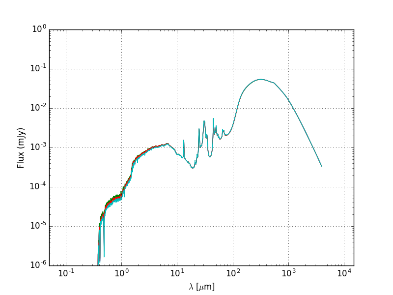
and an example plotting code can be found in the convenience subdirectory of the powderday root directory.
The individual parameter files that control this simulation are the parameters_master file and the parameters_model file. The descriptions of these are detailed here but in short, the parameters_master file is meant to control paramters that one might like to remain constant typically for every single galaxy in a given snapshot, or every snapshot in a model simulation. In contrast, the parameters_model file has variables such as the snapshot name, or output file name - variables that one might expect to change for different galaxies in a snapshot or different snapshots in a simulation.
Imaging
We can create monochromatic images by running the code in the exact
same manner as above, though setting the flag “IMAGING” to true in the
parameters_master file. A procedure to plot an image is demonstrated
in the convenience script make_image_single_wavelength.py, found
in the convenience subdirectory.
If filters other than the default filter (arbitrary.filter) are used,
powderday will convolve the
monochromatic image outputs with each filter’s transmission function and save
the result in the output directory as convolved.XXX.hdf5.
Say we’ve set the following in the parameters master file:
powderday will run at each wavelength in all of the specified filter files, and produce convolved image data for each filter.
After running:
>pd_front_end.py examples/gadget/mw_zoom parameters_master_401 parameters_model_401
we get the standard output files, along with the convolved image data (in this
case, it is named convolved.134.hdf5).
To load in the image data, use:
import h5py
f = h5py.File('convolved.134.hdf5', 'r')
Now, the image and filter data can be accessed in the hdf5 file format (thoroughly described in the h5py documentation).
Image data is stored in a 3-dimensional array, with the first axis across the
filters. The image’s index is matched to its respective filter filename, stored
in the filter_names dataset in the np.bytes_ format. So, if you wanted
to access a convolved image and its corresponding filter name, you could do:
>>> convolved_image = f['image_data'][0]
>>> filter_name = f['filter_names'][0].astype(str)
>>> print(filter_name)
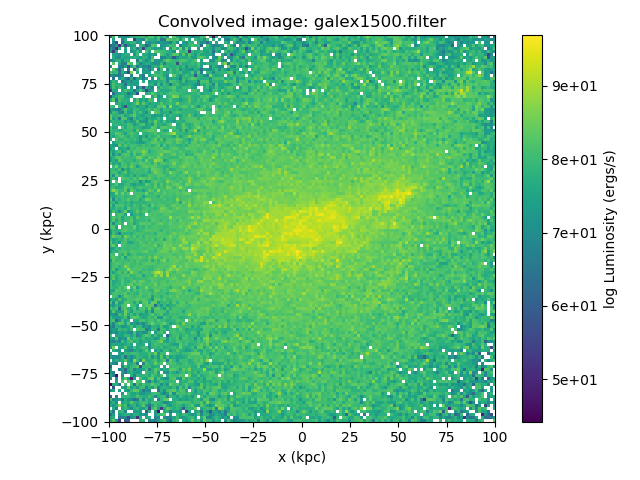
'galex1500.filter'
The filter’s transmission function must be accessed differently. Each filter’s transmission function is saved in its own dataset and can be called using its name:
>>> f['galex1500.filter'][...]
array([[ 1.3406205e-01,  9.0700000e-07],
       [ 1.3504851e-01,  1.1537571e-01],
       [ 1.3702143e-01,  1.7650714e-01],
       ...
The image width (float) and its units (np.bytes_ string) are stored as
attributes of the image_data dataset. To plot an image, one might do
something like this:
import matplotlib.pyplot as plt
import numpy as np

fig = plt.figure()
ax = fig.add_subplot(111)

w = f['image_data'].attrs['width']
w_unit = f['image_data'].attrs['width_unit'].astype(str)

cax = ax.imshow(np.log(convolved_image), cmap=plt.cm.viridis,
                origin='lower', extent=[-w, w, -w, w])
ax.tick_params(axis='both', which='major', labelsize=10)
ax.set_xlabel('x ({})'.format(w_unit))
ax.set_ylabel('y ({})'.format(w_unit))
plt.colorbar(cax, label='log Luminosity (ergs/s)', format='%.0e')
plt.title("Convolved image: {}".format(filter_name))
plt.tight_layout()
plt.show()